
Overview
One of the challenges for biomaterial application is to manufacture large scale protein production economically and efficiently. In our model, we integrated several levels of modelling to optimise the productivity of the whole system.
For our biomaterial production, we use split intein technology instead of genetic modification to gain longer protein polymers. Split inteins have a specific working temperature and pH condition for sufficient reaction rate. In our models, in addition to basic cell growth and protein expression model, we introduce intein polymerisation model (WORM) and fiber mechanical property simulation. Integrating these models, we can estimate the time required for desired protein polymerisation and thus provide the fiber with strong mechanical properties.
Cell Growth and Expression
Verhulst and Pearl and Reed played a huge part in developing a theory on logistic population growth. The rate considers an additional inhibition factor proportional to x2 from the Malthus population model.
This Riccati equation can then be solved analytically into:
We fit our data into the first-order ordinary differential equation model, and the sigmoidal curve that we get has a property of stationary area which is determined by 1/b.
| Symbols | Values and Units | Descriptions |
|---|---|---|
| t | hr | Time |
| x | dimensionless | Optical density of a cell at 600 nm wavelength |
| b | dimensionless | Inhibiting factor, which is inversely proportional to maximum cell population size. |
| k |
|
Population growth rate |
We determined the better growth media from the two broth we had available, which were Terrific Broth (TB) and Lysogeny Broth (LB).

The fitted equations tells us the inhibiting factor b for TB and LB, which are 0.3 and 0.4077, respectively. This is as predicted because TB has less inhibition compared to LB because of the nutrient abundance, carrier capacity, and toxicity level caused by the waste side-products of the cells. The same trend is also observed in maximum population, that TB provides a better environment for larger cell population in longer cultivations. Meanwhile for earlier growth rate k, cells in LB grow quicker before achieving stationary phase, which is 0.44hr-1 compared with 0.24hr-1 in TB.
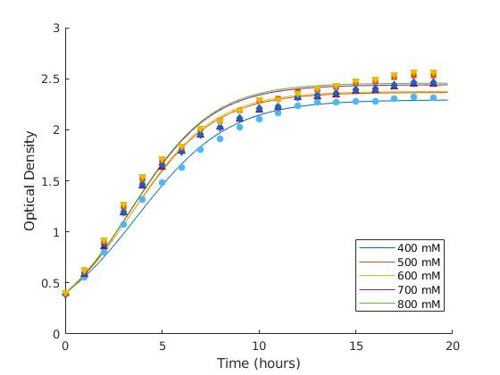

| IPTG Conc. | 400mM | 500mM | 600mM | 700mM | 800mM |
|---|---|---|---|---|---|
| k | 0.4215 | 0.4649 | 0.4735 | 0.4773 | 0.4759 |
| b | 0.4361 | 0.4227 | 0.4208 | 0.4097 | 0.4069 |
We then build up the kinetics inside a cell and integrate it with lab data analysis to understand protein production and get an effective lab plan for our E. coli system. GFP, RFP, and Intein Passenger fluorescence data of 544/590 nm filtering wavelengths were then extracted and processed. Each dependent value is described as protein-fold change post induction, which is normalised with the same system but uninduced, based on the fraction below:
The first-order system of linear differential equations are:
The first equation represents the mRNA system in a cell with the assumption of constant gene concentration in each cell. Meanwhile the latter equation is the protein system which is dependent on the previous equation, and fitted to the data from the plate reader, using the Trust Region Algorithm with non-negative floating number as the boundary in each parameter.
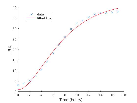
| IPTG Conc.(mM) | 400 | 500 | 600 | 700 | 800 |
|---|---|---|---|---|---|
| x | 200 | 200 | 200 | 200 | 200 |
| α | 0.02073 | 0.02332 | 0.02348 | 0.02156 | 0.02264 |
| β | 0.2482 | 0.2644 | 0.2642 | 0.2665 | 0.2777 |
| γ | 0.6564 | 0.6799 | 0.6668 | 0.7346 | 0.7449 |
| δ | 0.2563 | 0.2744 | 0.2719 | 0.2738 | 0.2827 |
| Symbols | Units | Descriptions |
|---|---|---|
| t | hours | Time |
| x | 200 | Plasmid copy number of pSB1C3 in each cell |
| m | dimensionless | Respective normalised mRNA concentration in each cell |
| p | dimensionless | Respective normalised protein concentration in each cell |
| α | hr-1 | Gene transcription rate or mRNA production rate |
| β | hr-1 | mRNA degradation rate and dilution factor |
| γ | hr-1 | Protein translation rate |
| δ | hr-1 | Protein degradation rate and dilution factor |
The α and β terms generally stay constant without a trend between IPTG concentrations which is explainable even though IPTG affects cell transcription activity. Since mRNA has a high rate of synthesis and degradation, it reaches equilibrium immediately as its stability closely follows inversely proportional to the mRNA concentration in the cell. The parameter γ and δ give a small yet noticeable increasing trend in higher IPTG level, this is related to protein concentration equilibrium, but not to the extent of mRNA degradation rate since protein relatively ‘lives’ longer than mRNA.
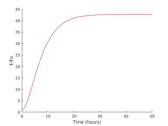
Generally IPTG does not give significant differences in high concentrations, so we chose 500 mM of IPTG which the model suggests as the most efficient with the similar expression level compared to the cells with higher concentration of IPTG. Further improvements of this model might include larger choices of medium and wider range of IPTG concentrations, together with cost analysis as it is an important factor in the larger scale production.
Protein Polymerisation
To better accommodate the integrated model and identify bottlenecks, we further develop a model entirely of in vitro polymerisation as it is indispensable to the overall process of biopolymer production.
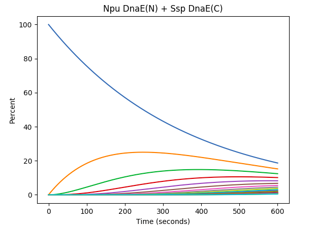
Each single protein is interpreted as a monomer with an irreversible polymerising capacity until it reaches an assumed maximum size. Polymer formation rate of each species (Pn) were then modelled in Python and plotted. The first term describes the polymer species formation from the sum of all reactions in the range of its possible constituents, and the second term represents the further polymerisation of the respective species as a substrate, which build up into larger repeats.

| Symbols | Values and Units | Descriptions |
|---|---|---|
| t | s | Time |
| n | dimensionless | Number of repeats, defining a certain species of polymer |
| Pn | mol L-1 | Polymer species n |
| k | L mol-1 S-1> | Rate constants of Intein activity of a certain intein |
| nmax | dimensionless | Maximum repeat number in a polymer |
Basically each intein rate of reaction (k) differs with each intein system we use.
| Intein | Rate of reaction (s-1) |
|---|---|
| Npu DNA-E | 1.1x10⁻² |
| SspDNA-E | 3.3x10⁻⁴ |
| Npu DNA-E(N) + SspDNA-E | 2.8x10⁻⁵ |
| SceVMA | 2.0x10⁻³ |
| SspDNA-B | 9.9x10⁻⁴ |
The results we get from the example runs of Npu DnaE(N) and Ssp DnaE(C) intein combinations are after 10 minutes of the simulated experiment, only 3.45% of monomers are in the form of the top 25% longest polymer species. However for Ssp DnaE inteins, in the course of 10 minutes, 72.3% of the monomers are polymerised into the same top 25% of the longest polymer region. This really shows how the intein polymerisation will require much less time compared to the cell culture and protein production. Further improvements will be introducing more parameters into the estimation function to represent more accurate results.
Intein Polymerisation
W.O.R.M.
To further model the polymerisation of our proteins, we devised a simplified proof of concept of our project using reporter proteins RFP and GFP to predict the polymerisation capabilities of split inteins. Each reporter protein is flanked by orthogonal inteins, which match up to the other reporter’s inteins to allow RFP and GFP to continuously link up into various lengths of polymers.
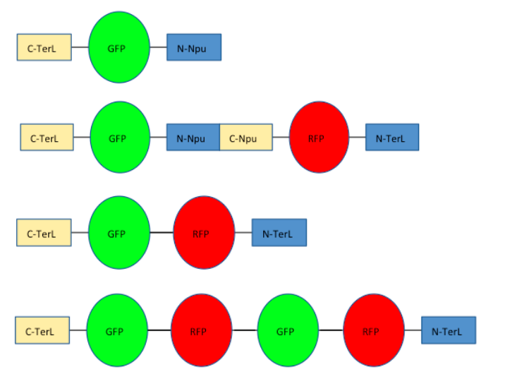
We used the python libraries PyGame and PyMunk to create an animated and interactive agent-based model of intein polymerisation. Acronymed WORM, this model depicts a Wonderful Oligomerisation Reaction Model.
Depicted in the video is a snapshot of the model WORM that shows intein polymerisation. The yellow and orange rectangles represent an split intein pair, as do the blue and cyan rectangles. The red and green rectangles represent the reporter proteins, RFP and GFP, respectively.
As an agent-based mode, WORM was created based on the following rules:
- Particles diffuse with random angular and lateral velocity;
-
Velocity increases with temperature (based on average kinetic energy):
Where:
- m= mass (kg)
- v= velocity
- k= Boltzmann constant
- T= temperature (K)
- Like reacts with unlike (RFP reacts with GFP);
- Particles are polarised (Npu-N [A1]→ Npu-C [B3], TerL-N [B1]→ TerL-C [A3]);
- Splicing removes 1+3 on reaction (removes the inteins);
- Steric hindrance by particles.
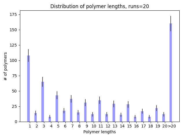
The interactive components of the WORM model include user’s choice of temperature and protein mass to selectively model the reaction conditions and functionalized protein of interest. These applications can be used by running the code found in our GitHub. The combination of predictive experimental data and the visually appealing computational model makes a user friendly platform for the public to better understand biology and modelling.
Mechanical Simulation
In this part, we also modeled the biomaterials’ micro-structure of the coarse-grained system. We predicted the structure of different spider silk repeats (tetramer, octamer and dodecamer) both after stretching and shearing. This method is a deterministic approach to foresee the network structure of spider silk repeats prior to the actual lab experiment and helps us to understand the design of the actual protein that we are going to produce afterwards.
Here is our initial designed sequence, a spider silk protein in repeats of four:
GQGGYGGLGSQGAGRGGLGGQGAGAAAAAAAAGGAGQGGYGGLGSQGAGRGGLGGQGAGAAAAAAAAAGGYGGLGSQGAGRGGLGGQGAGAAAAAAAAGGAGQGGYGGLGSQGAGRGGLGGQGAGAAAAAAAAGGA
The respective sequence is then quantitatively analysed for their hydrophobicity and hydrophilicity and plotted.
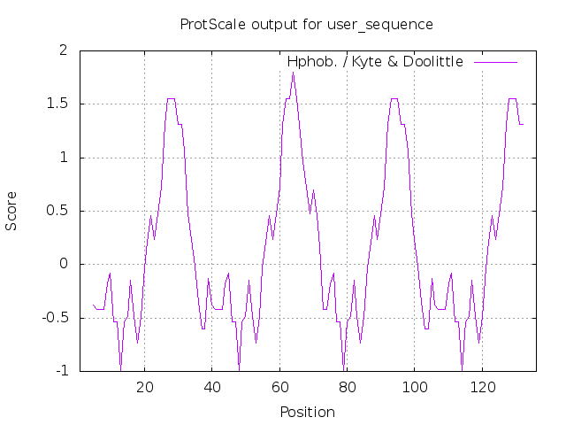
In this particular sequence, we can observe that the hydrophobic and hydrophilic parts alternate inside the spider silk fiber, which will form aggregates and bridge connections to achieve desired tensile and toughness due to the hydrophobic interactions.
This alternating pattern seen in the figure allows us to simplify proteins as the hydrophobic domains and hydrophilic domains. These domains are then represented as a collection of the so-called ‘beads’, and depending on relative molecular volume of each domain, the coarse-grained model is then scaled and measured into an estimate of three amino acid residues per bead.
This system is composed from 3 components: water, hydrophilic and hydrophobic beads. Every 9 water molecules is represented as a single bead, so its 270 Å size (each water molecule is about 30 Å) is proportional to the protein beads.
We then introduce LAMMPS as our software, which is an abbreviation of Large-scale Atomic/Molecular Massively Parallel Simulator, to simulate the behaviour of our ‘beads’ collection in a single compartment and thus gave us an insight into the physical property of the recombinant spider silk.
Simulations
Hover to compare the 2 sides.
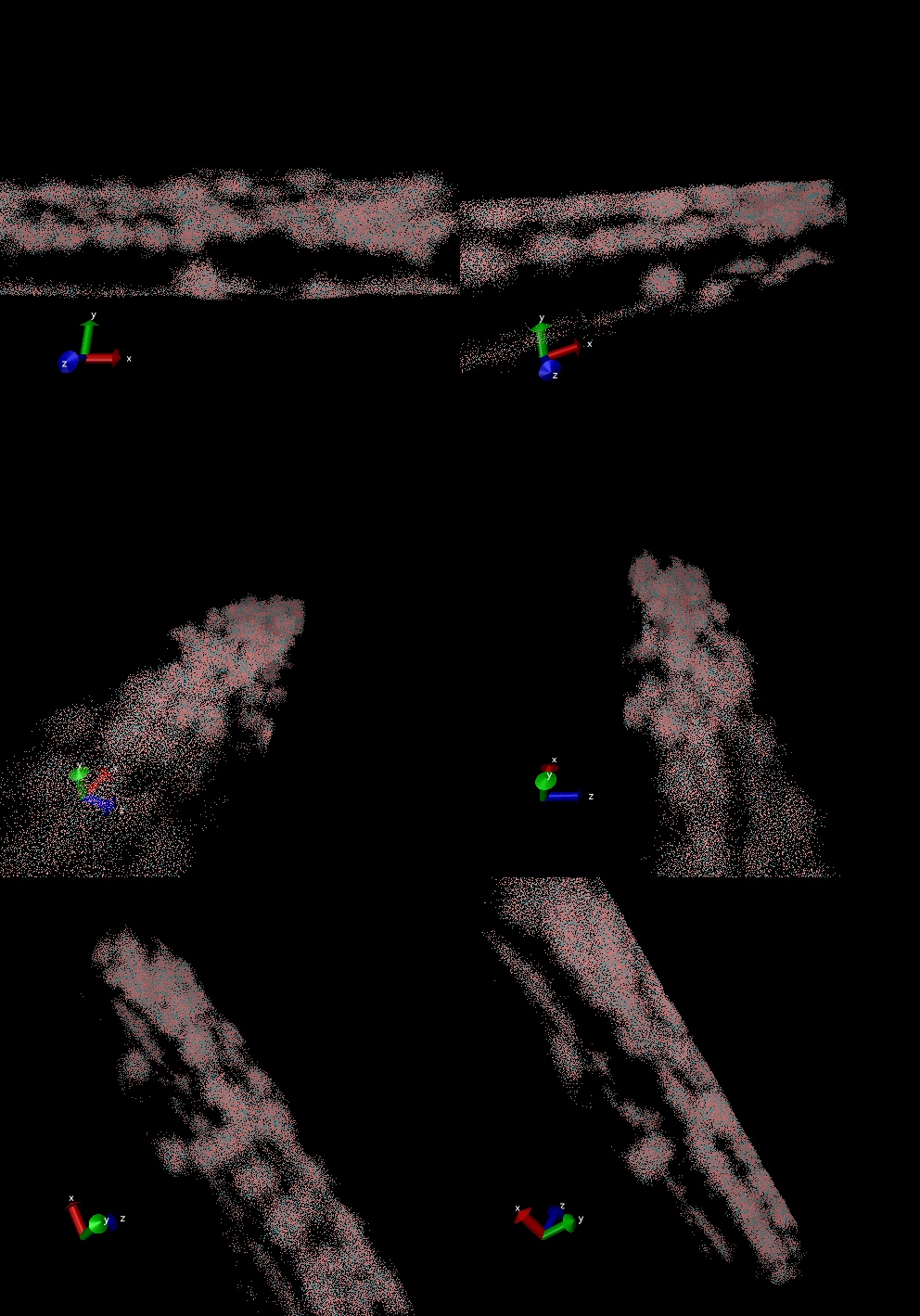
Tetramer
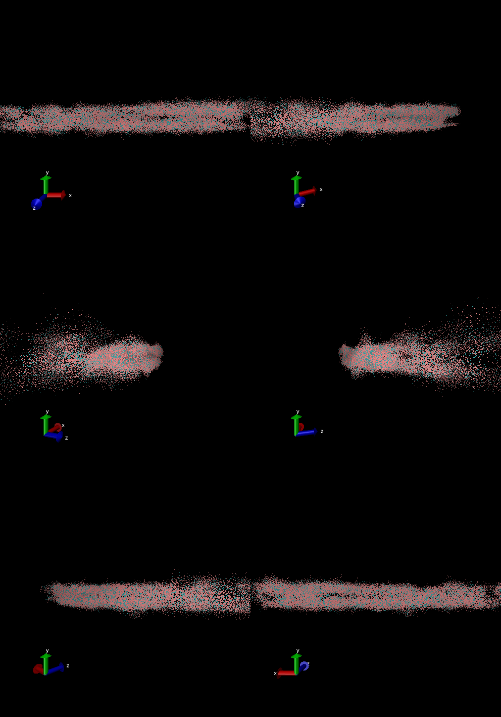
Octamer

Dodecamer
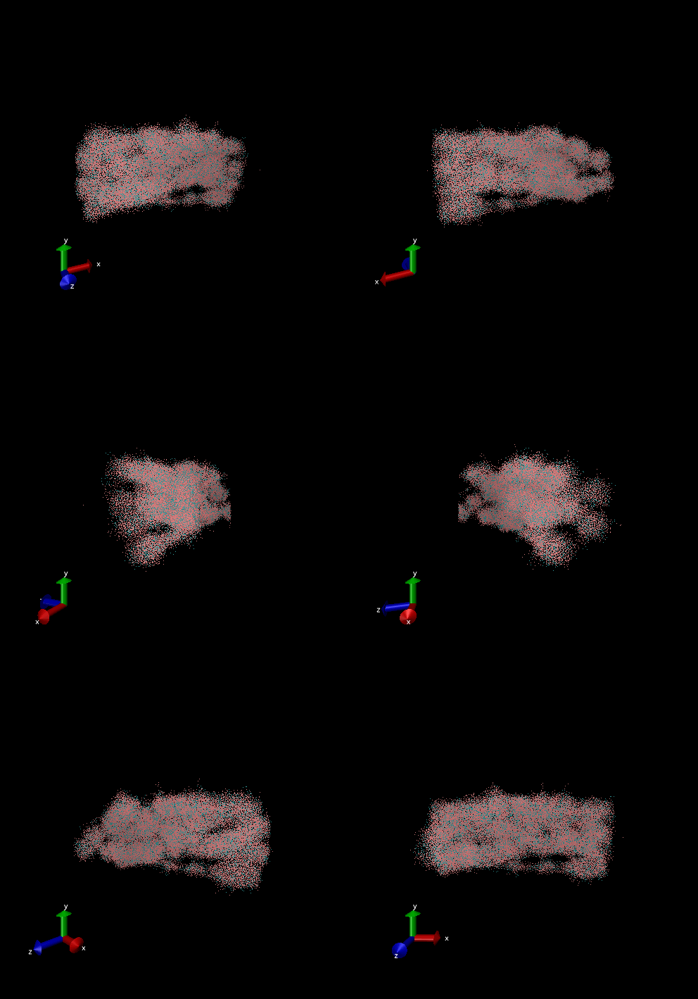
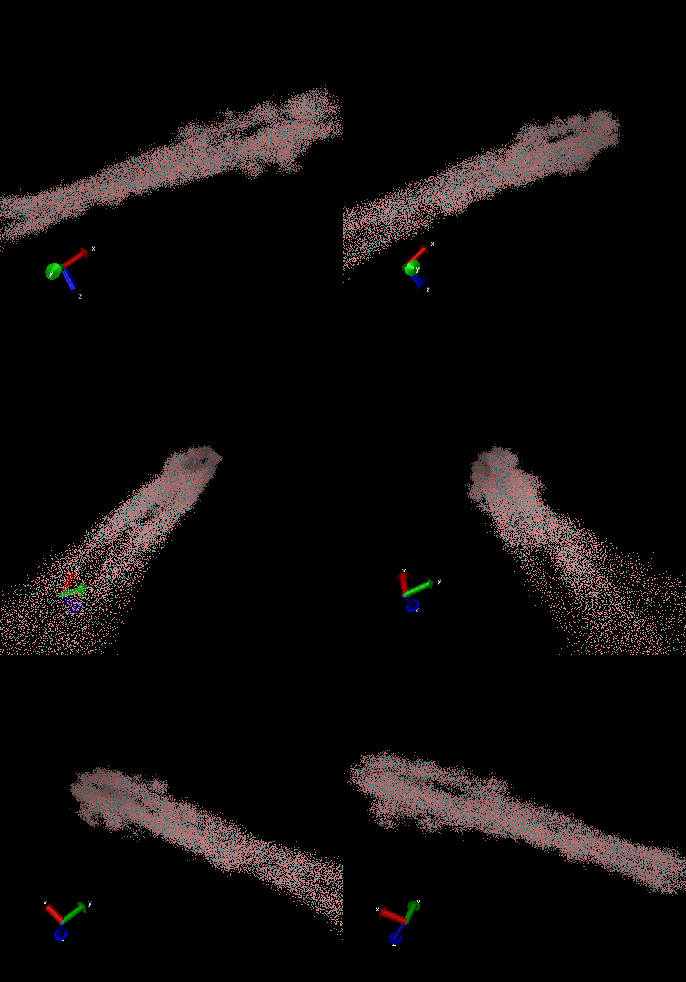
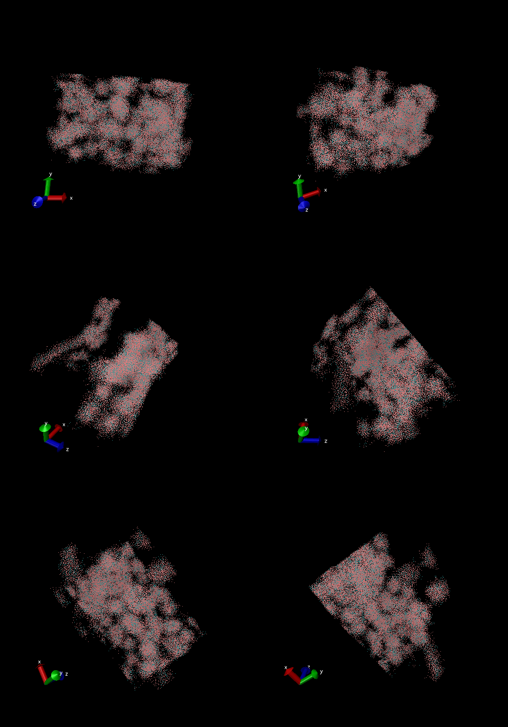
For these simulation results, the configurations of spider silk fiber after applying a constant engineering strain rate (7.5 × 10⁻⁶ τ-1 along the x-axis) and at equilibrium after shear flow (0.01 τ-1 along x axis for 420000 shear steps). The red nodes show hydrophobic aggregated protein clusters and the blue lines are the bridge connecting two clusters. Uniform distribution and high density of clusters and bridges represent the better mechanical property, higher tensile and toughness. For stretch testing. we can analyse the tetramer structure which consists of large and frequent cavity in the fiber. The octamer and dodecamer is predicted to be able to tolerate this strain, which means they have a considerable threshold of mechanical strain. In order to examine which structure is the best, we apply shear flow. In this case, it is observed that only the dodecamer still keeps its original structure but others break at different levels. In conclusion, dodecamer is the best configuration required in making desired fibers.
Bibliography
- Verhulst PF. Notice sur la loi que la population poursuit dans son accroissement. Correspondance mathématique et physique. 1838;10:113–21.
- Pearl R, Reed L. On the Rate of Growth of the Population of the United States since 1790 and Its Mathematical Representation. Proceedings of the National Academy of Sciences. 1920;6(6):275-288.
- Bailey J, Ollis D. Biochemical engineering fundamentals. 2nd ed. New York: McGraw-Hill; 1944.
- Part:pSB1C3 - parts.igem.org [Internet]. Parts.igem.org. 2008. Available from: http://parts.igem.org/Part:pSB1C3
- Zettler J, Schütz V, Mootz HD. The naturally split Npu DnaE intein exhibits an extraordinarily high rate in the protein trans-splicing reaction. FEBS Letters 2009;583:909–14.
- Nichols NM, Benner JS, Martin DD, Evans TC. Zinc Ion Effects on Individual Ssp DnaE Intein Splicing Steps: Regulating Pathway Progression. Biochemistry 2003;42:5301–11.
- Al-Ali H, Ragan TJ, Gao X, Harris TK. Reconstitution of Modular PDK1 Functions on Trans-Splicing of the Regulatory PH and Catalytic Kinase Domains. Bioconjugate Chemistry 2007;18:1294–302.
- Brenzel S, Kurpiers T, Mootz HD. Engineering Artificially Split Inteins for Applications in Protein Chemistry: Biochemical Characterization of the Split Ssp DnaB Intein and Comparison to the Split Sce VMA Intein. Biochemistry 2006;45:1571–8.
- Kyte J, Doolittle RFA. simple method for displaying the hydropathic character of a protein. Journal of Molecular Biology. 1982;157(1):105–32.
- ExPASy - ProtScale [Internet]. Web.expasy.org. Available from: https://web.expasy.org/protscale/
- Rim N, Roberts E, Ebrahimi D, Dinjaski N, Jacobsen M, Martín-Moldes Z, Buehler M, Kaplan D and Wong J. Predicting Silk Fiber Mechanical Properties through Multiscale Simulation and Protein Design. ACS Biomaterials Science & Engineering. 2017;3(8), pp.1542-1556.
- Lin S, Ryu S, Tokareva O, Gronau G, Jacobsen M, Huang W, Rizzo D, Li D, Staii C, Pugno N, Wong J, Kaplan D and Buehler M. Predictive modelling-based design and experiments for synthesis and spinning of bioinspired silk fibres. Nature Communications. 2015;6(1).


